Journal Name: Journal of Health Science and Development
Article Type: Research
Received date: 18 October, 2021
Accepted date: 09 December, 2021
Published date: 2024-02-01
Citation: Mastmeyer A, Zettler N (2021) Abdominal Organ Segmentation in 3D CT images using 2D vs. 3D U-Nets. J Health Sci Dev Vol: 4, Issue: 2 (43-50).
Copyright: © 2021 Mastmeyer A et al. This is an open access article distributed under the terms of the Creative Commons Attribution License, which permits unrestricted use, distribution, and reproduction in any medium, provided the original author and source are credited.
Abstract
We introduce a two-stage approach for 3D segmentation of 5 abdominal organs in volumetric CT images. First, the relevant volume of interest for each organ is extracted as a bounding box. The obtained volume serves as input for a second step, in which two U-Net architectures of different dimensionalities are applied to reconstruct an organ segmentation as a label mask. The focus of this work is on the comparison of 2D U-Nets vs. 3D U-Nets counterparts. Overall, the results of our study show Dice improvements of at most 6%. Regarding computation time, to our surprise, the segmentation of liver and kidney was performed significantly faster by the GPU memory-saving 2D-U Nets. There were no significant differences for other major abdominal organs, but for all organs tested, we observe highly significant advantages for the 2D U-Net in terms of GPU computational effort.
Keywords:
Organ bounds; U-Net; Architecture; Abdomen; Segmentation; 3D CT images.
Introduction
Steady progress in the field of deep learning and artificial intelligence is opening up previously unimagined possibilities for medical research. However, even with the increasing availability of publicly accessible databases, the automated just-in-time (JIT) segmentation of 3D patient organ models remains an unsolved challenge. As manual segmentation of abdominal organ structures in axial CT slices is a very time consuming task, automatic and JIT reconstruction procedures of 3D models are highly relevant for surgery planning and navigation.
Over the years, various Convolutional Neural Network (CNN) models for image segmentation have emerged, some of which differ greatly in memory requirements and the saving of computational power. In 2015, the 2D U-Net architecture showed promising results that outperformed conventional models on 2D biomedical segmentation problems and was also found to be effective on lower resolution images [1]. In contrast to the previously known CNN models, the U-Net concept uses downand up-sampling steps to resample the condensed feature map to the original size of the input image. With the inclusion of higher resolution feature information in each up-sampling step, semantic segmentation of the input images can be accomplished efficiently by skip connections. In 2016, the resulting U-shaped architecture was extended to a 3D U-Net edition by Cicek et al. by replacing 2D operations with their 3D equivalents [2]. The primary focus in this paper is to address the question of whether the 3D U-Net is truly better suited for 3D data.
We expect that in Big Data studies, parallel segmentation of thousands of 3D volumetric images requires high computational time due to the limited amount of processing nodes and sub-processes for parallel processing. We conjecture that 3D U-Nets will require even higher GPU computational and memory overhead for 3D image processing. In this work, we focus on proposing solutions with the lowest possible cost while maintaining or even improving segmentation quality. The goals of our approach can be summarized in three simple steps:
We detect and apply U-Nets to local sub-images for each task (liver, kidneys, spleen, pancreas).
We compare two U-Net architectures in terms of quality and GPU-performance when executing semantic segmentations.
We recommend the more suitable architectural model to the interested reader based on a detailed statistical analysis.
Finally, using an image database of 80 CT scans and their ground truth segmentations, the question whether the simpler 2D U-Net might perform better than the complex and theoretically more powerful 3D U-Net will be answered.
Particularly in the emerging field of visuo-haptic training and planning interventions using virtual reality (VR) techniques, fast and accurate 3D segmentation results are of utmost importance [3-6]. Time-variant 4D VR simulations with breathing simulation are readily available for training and planning of liver needle interventions [7-11]. A major obstacle remains the JIT and high-quality reconstruction of all required 3D models, i.e., abdominal organs in particular are rarely easy to segment. This is due to varying imaging conditions such as contrast agent administration, structure variations and noise.
In the literature, 3D U-Nets are often suggested to be more powerful [12-16]. However, there are some studies that highlight the advantages of 2D U-Nets in 3D segmentation tasks, such as [17-19]. Nemoto et al. find that 2D U-Nets with low computational complexity are effective and equivalent to 3D U-Nets for semantic lung segmentation, except for the trachea and bronchi [17].
A hybrid approach of 3D and 2D inputs for evaluating hemorrhage on CT scans of the head was proposed by Chang et al. [20]. This method was later adapted by Ushinsky et al., applying it to segmentation of the prostate in MRI images, demonstrating that 2D U-Nets are very effective for 3D data [19]. Christ et al. provided a slice-wise application of 2D U-Nets for liver segmentation in combination with 3D random fields [21]. Similarly, Meine et al. proposed liver segmentation methods with the assistance of 3D, 2D and three fused 2D U-Net sectional (axial, coronal, sagittal) results in a 2.5D ensemble approach [18]. They find that the 2.5D U-Net ensemble results are statistically superior for liver segmentation, especially for images with pathologies.
Other recent approaches aim to combine multiple stacked 2D U-Nets and further improve information flow through semantic connections between different components [22,23]. The same concept has also been used in application areas such as colon polyp segmentation and face recognition [24,25]. Zwettler et al. have recently shown that extending datasets with synthesized slices can notably improve the results of 2D U-Nets applied on a small number of training datasets, indicating further potential for the 2D approach [26].
Regarding our 2D U-Net setup for the abdominal organs liver, spleen, kidneys and pancreas, we prefer axial slice training within the previously determined organ-specific VOIs. This results in significant savings in radiation dosage savings due to high scan pitch. Yet image resolution in axial CT slices is very high. New aspects in this work include the organ-specific VOI approach for the investigated organs such as liver, spleen, kidneys and pancreas. Finally, an organ-specific architecture dimensionality recommendation is given for each of the organs.
Materials and Methods
For the training and testing of our U-Nets, eighty CT scans and the corresponding labeled images were used, which can be found in various public sources1. Besides differences in image information in terms of quality, noise, and field of view, patient-specific volume representation also varied in the number of slices (64 to 861), pathologic lesions, slice width (1 to 5 mm), and contrast agent used.
The main problem concerning data annotation was the weakly contrasted pancreas organ in the CTs, which was not present in some image sets consisting of congruent intensity and label images from the public sources. We coped with that by four eye reviewed manual segmentation of this occasionally missing structure in the label maps. However, most organ reference segmentation were readily available in the public data sources.
Data preparation
To ensure a fair processing of the data, the orientation of images was changed to Right-Anterior-Inferior (RAI) and zero origin (0.0, 0.0, 0.0). Because CNNs are not able to natively interpret voxel spacings, an isotropic image resampling with 2.03 mm was performed as a compromise for varying xyz-distances (xy ≤ 2 mm, z ≤ 5 mm).
Our approach consists of two different machine learning techniques, bounding box detection using random regression forests (RRF) and U-Nets for semantic segmentation. After using the RRFs to detect the organ VOIs in the CT data, the U-Nets are applied to segment the organs contained in the VOIs.
Volume of interest detection
For the evaluation of this work, the ground truth of the corresponding organ VOI bounding box (BB) is required. It can be created by scanning the reference segmentation maps for labeled voxel coordinate extremes. To create a three-dimensional BB vector for each organ, we iterate in orthogonal slices through the organ’s label map for each coordinate direction (x, y, z) and store the extreme limits in a 6D BB vector that functions as ground truth BBs.
Alternatively, VOI-based organ extraction is readily available for organ-specific VOI detection of the organ ensemble (liver, still left kidney, right kidney, spleen, pancreas) [27-29]. This step also solves the FoV problem in the z-direction of the scanner, since CT scans cover variable body portions. Our currently studied scheme for learning bounding boxes of VOIs using RRFs is summarized below.
Training and application of random regression forests
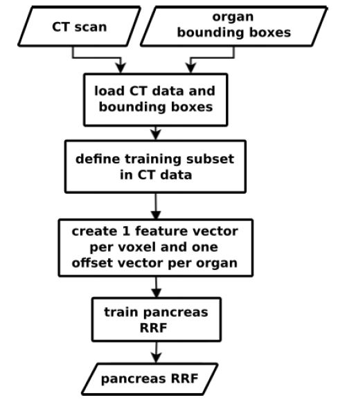
We use Random Regression Forests (RRF) to determine the location and extent of abdominal organs [29]. As shown in figure 1, the RRF training step expects scans and ground truth VOIs as input.
A three-dimensional VOI bc of an organ c can be described by using a 6D vector with coordinates in mm [29]. To reduce the amount of data and speed up the algorithm runtime, only a fraction of the voxels in the scan is used for bounding box calculation. Starting from the scan center, we calculate the position of the voxels in each axis direction that are 15 mm away from the center, forming a cuboid box around the center. All voxels inside this area are part of the subset used for training and application of the algorithm.
Feature and offset vector calculation
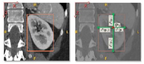
Each voxel in the subset is assigned a feature and an offset vector. As described in eq. 1, the offset vector of a voxel is the difference d(p,c)=p-bc
between its position and the position bc of eachof the six bounding box walls of the organ. Figure 2 shows this principle on the example of a kidney.
Figure 1:The inputs for the training process are CT scans and ground truth VOIs of a targeted pancreas. We create one feature vector and one mm offset vector for each voxel that is part of a predefined medial cylinder subset in the scan [29]. The trained RRF is able to predict the offset between a voxel and an organ’s VOI walls.
The feature vector of a voxel is derived from several feature boxes generated by traversing the voxels that are within a specified radial distance (r = 5 cm) from the scan medial axis. By computing the average intensities of all feature boxes obtained, the aim is to capture the spatial and intensity context around the voxel. Eq. 2 describes the calculation of a feature vi;
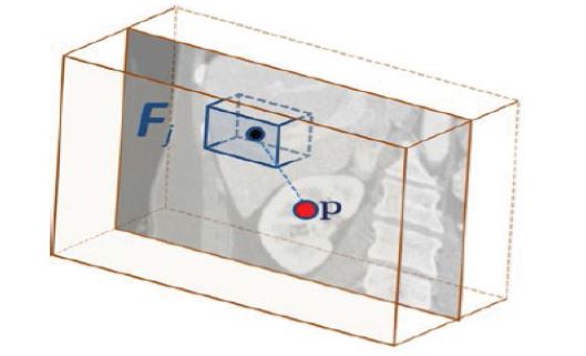
Fp;i represents the feature box of the ith feature, q indicates the points inside Fp;i and J (q) determines the intensity at position q. The feature box is defined related to the current voxel. In contrast to Criminisi et al. [29], we use only 50 feature boxes, that are evenly distributed on three spheres (r = 5 cm, 2.5 cm, 1.25 cm). The input feature vector is finally composed of the mean intensities of the feature boxes. Figure 3 shows an example feature box, that was created in correlation to the selected voxel.
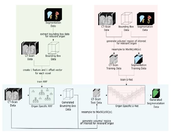
During the first step of our application scheme (figure 4, left), the RRF localizes the VOI for each individual organ as BB. Finally, the information of a detected VOI (intensities, labels) is resampled to 96x96(x96) for CNN input (figure 5).
Training and application of 2D and 3D U-Net architectures
In the second stage, as shown in the bird’s eye view in figure 4, right, the resulting VOI is passed to either a 2D [1] or a 3D U-Net for semantic labeling [2].
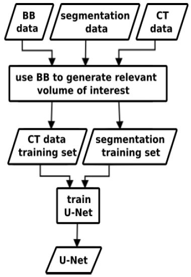
The training data for our U-Net is composed of the expert segmentations and ground truth bounding box interiors, as shown schematically in figures 6,4. The VOIs are then used to locally extract the intensity and label data from the CT scans. As input, a U-Net obtains a VOI from the intensity data, whereas the corresponding label data is linked to the output. We use slightly modified 2D and 3D U-Net architectures compared to Ronneberger et al. [1].
U-Net architecture overview
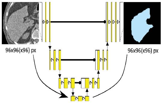
As can be seen in figure 5, our architecture consists of four down- and up-scaling steps that act as analysis and synthesis paths. Skip connections between the corresponding levels allow for the incorporation of additional information in the form of high-resolution features at each up-scaling step. Starting with the VOI input of size 96x96(x96), each downscaling step consists of two 3x3(x3) convolutions with a small dropout layer in between to prevent overfitting. Each step is then followed by a 2x2(x2) max-pooling layer until the final down-scaling step. In the up-scaling path, each step is introduced by a 2x2(x2) transposed convolution, which is then concatenated with the skip connection output from the corresponding down-scaling step. The last step is followed by a 1x1(x1) sigmoid activation function that provides the final segmentation result. For the 3D U-Net, an additional layer depth dimension is added while all other design elements are kept constant.
By using the data contained in a given VOI bounding box to segment the corresponding organ, the resulting output is a local segmentation map of the entire target organ in a probability range of 0 to 100%. The threshold for all organs except pancreas was chosen as 50%. For pancreas 30% was empirically found best.
Figure 2:Offset vector between bounding box and voxel [29] on the example of a kidney. Left: Position of a bounding box around the kidney corresponding to the extreme values of the organ in each axis direction. Right: Position of a voxel p with the distance vectors d(p,c) to each of the bounding box sides.
Figure 3:Example of a feature box [29]: The feature box Fj corresponds to the current voxel p and calculates the mean value of a 3D image section. By sampling multiple feature boxes within a specified radius, the spatial environment of p can be described.
Figure 4:Bird’s eye perspective on our current segmentation concept with RRF for VOI detection and subsequent U-Net. Both training (green, red) and application (blue) concepts are shown. In this work, the right part with regards to the U-Nets is focused in the evaluation.
The U-Nets were trained with batches of size 8 over 100 epochs. In addition, Adam optimization and a cross entropy loss function were used. A separate U-Net is trained for each organ, using a ReLU activation function.
Evaluation, metrics and statistics
To allow for a fair comparison, we use the same 64 training images for both U-Nets in each iteration of the crossvalidation and perform testing with the same 16. In this way, we avoid data contamination due to separate training and test sets. The only difference between the U-Net architectures is the dimension of the input, output, and filter kernel layers. For 2D U-Nets, the input and output dimensions are 96x96 and 2D filter kernels are applied in the layers. Respectively, for 3D U-Nets we have 96x96x96 inputs and outputs and apply 3D convolutions in the architecture layers.
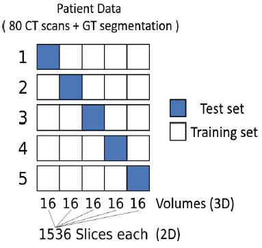
A 5-fold randomized cross-validation using 4:1 splits was used. Five iterations yield 80 quality measures for each organ used in our statistics (table 1). This means that five new models for each organ are trained with randomly selected training data and used in the analysis. Figure 7 illustrates the partition of training and testing data. To focus solely on the influence of the U-Net dimensionality, the reference VOIs were used for the evaluation of this study. The Dice similarity coefficient was used as metric for the analysis:
Where, U is the set of voxels from U-Net object segmentation and G is the set of ground truth voxels. A DSC value of 1 indicates perfect segmentation, a value close to 0 implies poor segmentation. From the DSC results, we calculate means and standard deviations, medians and Inter-Quartile-Ranges (IQR) as measures of accuracy and precision. Statistical analyses with paired T-tests and Wilcoxon-Signed-Rank(WSR)-tests were performed using GNU-R 4.0.3. Finally, we recommend the dimensionality of the U-Net architecture based on accuracy, i.e. greater mean or median, and precision, i.e. smaller standard deviation or IQR and smaller number of outliers. We also keep in mind the relationship between quality and GPU overhead in time and memory.
Results
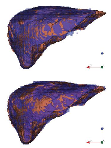
The qualitative liver results (figure 8) show that the 2D U-Net (top) is superior with more uniform coverage of the segmentation area. The 3D U-Net (bottom) obviously suffers from under-segmentation as more brown ground truth surface is visible in figure 8 (bottom). With reference to table 1, the precision of the 2D U-Net is also higher due to the lower std. deviations and IQRs.
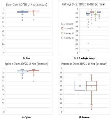
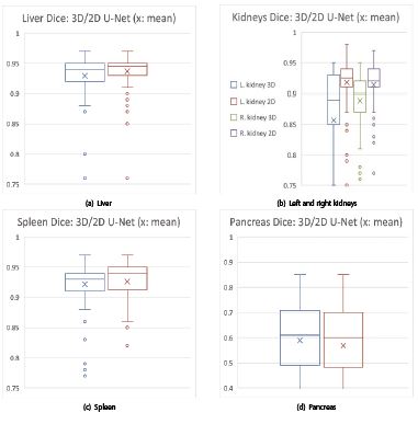
Regarding the kidney results, the 2D U-Net is highly significantly better in both T- and WSR-tests. The boxplots with a small x for the mean in figures 9, 10 visually confirm: the 2D U-Net is significantly better for liver and highly significantly better for kidneys (figures 9a, 10a, 9b, 10b).
For spleen segmentation, the 2D U-Net tends to have an advantage, as indicated in figures 9c, 10c and table 1.
The 3D U-Net has higher accuracy and precision for the low-contrast pancreas. The higher precision is reflected in smaller standard deviations and fewer outliers in table 1 and figures 9d and 10d. In terms of accuracy measured by medians, the 3D U-Net has trend advantage of 0.02 over the 2D U-Net, while precision measured by IQR is equal.
Table 1:Mean DSCs with standard deviations (Mean ± Std.) and Median DSCs with Inter-Quartile-Range (IQR) (Median~IQR) of 2D and 3D U-Nets from 5-fold randomized cross-validation experiments using 4:1 splits of the 80 images into training and test data.
| DSCs: Organ | Mean±Std. | Median~IQR | ||
|---|---|---|---|---|
| 2D U-Net | 3D U-Net | 2D U-Net | 3D U-Net | |
| Liver | 0.94±0.03* | 0.93±0.04 | 0.95~0.02** | 0.94~0.03 |
| R. kidney | 0.91±0.05*** | 0.89±0.05 | 0.92~0.03*** | 0.90~0.05 |
| L. kidney | 0.92±0.05*** | 0.86±0.14 | 0.93~0.03*** | 0.89~0.08 |
| Spleen | 0.93±0.04 | 0.92±0.04 | 0.94~0.03 | 0.93~0.03 |
| Pancreas | 0.57±0.19 | 0.59±0.15 | 0.60~0.21 | 0.61~0.21 |
| We use statistical standard notation for found significances: *; **; ***: p<0.05; p <0.01; p <0.001 from T-tests (paired) and Wilcoxon-Signed-Rank-Tests on the right of the favorable U-Net result. | ||||
Table 2:GPU-Performance table with memory consumption for training and application to the left and training and application times to the right.
| GPU-Performance: Organ | Memory | Time | ||||||
|---|---|---|---|---|---|---|---|---|
| Training [MiB] | Application [MiB] | Training [MiB] | Application [MiB] | |||||
| 2D U-Net | 3D U-Net | 2D U-Net | 3D U-Net | 2D U-Net | 3D U-Net | 2D U-Net | 3D U-Net | |
| Liver | 1693 | 10957 | 1693 | 9117 | 9:26 | 10:07 | 1.47 | 3.18 |
| R. kidney | 1693 | 10957 | 1693 | 9117 | 9:28 | 10:07 | 0.40 | 0.55 |
| L. kidney | 1693 | 10957 | 1693 | 9117 | 9:26 | 10:07 | 0.40 | 0.55 |
| Spleen | 1693 | 10957 | 1693 | 9117 | 9:27 | 10:08 | 0.40 | 0.55 |
| Pancreas | 1693 | 10957 | 1693 | 9117 | 9:28 | 10:08 | 0.40 | 0.55 |
| Mean±Std. | 1693±0*** | 10957±0 | 1693±0*** | 9117±0 | 9:27±0:01*** | 10:07±0:01 | 0.61±0.43 | 1.07±1.05 |
| Median~IQR | 1693~0*** | 10957~0 | 1693~0*** | 9117~0 | 9:27~0:01+ | 10:07~0:01 | 0.40~0.003+ | 0.55~0.001 |
| Mean Improvement | 647.19% | N/A | 538.51% | N/A | 107.13% | N/A | 175.22% | N/A |
| Median Improvement | 647.19% | N/A | 538.51% | N/A | 107.07% | N/A | 137.10% | N/A |
| 1 MiB=1.048581024 MB=10242 bytes. We use statistical standard notation for found significances: +; *; **; ***: p <0.10; p <0.05; p <0.01; p <0.001 from T-tests (paired) and Wilcoxon-Signed-Rank-Tests on the right of the favorable U-Net result.. | ||||||||
Figure 5:Simplified overview of the U-Net architecture used for both the 2D and 3D case. The input VOI of size 96x96(x96) is processed through four down- and up-scaling steps, resulting in a segmentation map of the same size as the input, containing organ pixels in the probability range from 0 to 100%. Applying a specified threshold leads to the final result.
The GPU-Performance evaluation in table 2 shows the superiority of the 2D U-Net at the scale of this study with an 80-image data base. The ratio of quality to GPU resources is always better for the 2D U-Net. In table 2 GPU memory saving is >6-fold in the training phase and >5-fold in the model application, trivially a highly significant result since there is no variation, i.e. no standard deviation and IQR. In terms of GPU calculation times measured during training, the 2D U-Net is exactly 40 seconds or 7% faster on average, again a highly significant average result. In the U-Net model application, we can observe a weakly significant ( p < 0.1) advantage for the 2D U-Net from 37% to 75%.
Figure 6:The inputs to the training process are ground truth bounding boxes VOIs, CT scans and their corresponding segmentation maps. The box crops the CT- and segmentation data to extract the relevant image region. Inside the organ VOIs, the segmentation is learned. The process results in organ-wise training and application of U-Nets.
Figure 7:5-fold randomized cross-validation with 4:1 splits of 80 CT scans and their ground truth segmentations. Each subset consists of 16 CT volumes for the 3D case, corresponding to 1536 slices for each set of the 2D case. Training set (white) and test set (blue) are changed in every iteration, so that after five iterations each subset was once the test set.
Figure 8:Two liver segmentations (anterior view) with 2D U-Net (top) and 3D U-Net (bottom). The coverage of the 2D U-Net result (top) appears more evenly distributed, i.e. more sensitive. Brown: Reference and purple: U-Net CNN. N.B., for the 2D model result on top, the oscillation pattern between reference (brown) and 2D CNN segmentation (purple) is much denser, showing better mean local quality. Legend: reference (brown) and U-Net segmentation (purple
Figure 9:Overview DSC boxplots: 3D (blue, green) and 2D U-Net (brown, purple) on the x-axis vs. DSCs on the y-axis: 2D U-Nets in favor for (a) liver and (b) kidneys (left k. and 3D U-Net: blue, left k. and 2D U-Net: brown; right k. and 3D U-Net: green, right k. and 2D U-Net: purple). (c) Spleen comes out with an edge for the 2D U-Net by trend. (d) Mixed results: 2D U-Net wins the accuracy contest, but loses the precision contest in terms of lower standard deviation (cf. tab. 1) and regarding less outliers for pancreas. Legend: for (a), (c) and (d): blue boxplots: 3D U-Net; red boxplots: 2D U-Net.
Figure 10:Zoomed DSC boxplots: 3D (blue, green) and 2D U-Net (brown, purple) on the x-axis vs. DSCs on the y-axis: 2D U-Nets in favor for (a) liver and (b) kidneys (left k. and 3D U-Net: blue, left k. and 2D U-Net: brown; right k. and 3D U-Net: green, right k. and 2D U-Net: purple). (c) Spleen comes out with an edge for the 2D U-Net by trend. (d) Mixed results: 2D U-Net wins the accuracy contest, but loses the precision contest in terms of lower standard deviation (cf. tab. 1) and regarding less outliers for pancreas. Legend: for (a), (c) and (d): blue boxplots: 3D U-Net; red boxplots: 2D U-Net.
Conclusion
Surprisingly in this study, 2D U-Nets are favorable regarding the ratio of quality vs. computing costs.
The liver and spleen hold the greatest volume in our abdominal organ group. The liver and especially kidney competition is significantly won by the 2D U-Net ( p < 0.05). The liver is a difficult organ often with a variably filled stomach as a neighbor.
Kidneys can be regarded as easy organs lighted by contrast agent and inside fatty tissue with low CT intensity.
A better posed training for the 2D U-Net could be the reason for the 2D U-Nets’ better results for liver and kidney tasks. A higher relative number training elements is used, i.e. axial slice pixels, vs. the number of net weights. The spleen results are in favor of the 2D U-Net regarding the mean and medians by trend. The 2D U-Net is also favorable for a less number of outliers (figure 9c).
The difficult pancreas does not provide many axial training slices useful for the 2D U-Net, as its elongation is not prominent on the z-axis. We suppose this is the reason, why and precision, i.e. higher mean and lower standard deviation and lower number of outliers (figure 9d). This win is supported by higher accuracy for the 3D U-Net in terms of medians. However, the race is not decided by significant differences making the 2D U-Net still very attractive for some users with GPU performance and memory concerns. Abdominal volumetric CT images and key organ segmentation were analyzed.
This new study shows interesting results from competing U-Net architectures, especially focusing different dimensionalities of net filter bank kernels and quality vs. GPU performance. The interested reader can now select a particular U-Net architecture, primarily whether to use a computational inexpensive design. Finally, in this study’s scope, a humble recommendation for the 3D U-Net could be given for the pancreatic organ in terms of better accuracy by trend and smaller standard deviation only. The IQRs as an alternative measure of precision are on par, and regarding the median the 3D U-Net wins just by a small trend. We coconclude, because of the deeper layering structure and thus more trainable weights, a 3D U-Net needs significantly more training data vs. possible overfitting to outpace 2D U-Nets.
As training volumes are normalized to a square or cube of 96 voxels, the GPU memory consumption in table 2 is always constant. Therefore, differences are trivially highly significant, as no varying results occur. We observe consistently lower memory consumption for 2D U-Nets. The memory effort in training is higher for the 3D U-Net including more space for administrative overhead data. Thus, 2D U-Nets can run on affordable 2-4 GB GPUs for 3D CT volume segmentation. 3D U-Nets definitely need currently totally overpriced 12 GB GPUs.
The timing measures in table 2 clearly speak out for the 2D U-Net. Training is highly significantly 40 seconds or 7% faster on average using the 2D U-Net. However, regarding application, in the trained model prediction, the differences are not so striking with a weak significance by median. 37% to 75% improvement can be achieved, however in the range of one second, which is practically unimportant.
As final and bold conclusion regarding our study design and results, we can recommend using the 3D U-Net subject to the amount of data we used here - for pancreas only. The conclusions are justified by statistically significant or by trend quality and GPU-computation performance results for all organs under study. We suppose, 3D U-Nets may overcome in quality when using several hundreds of training images. However, this comes approximately with an order of magnitude higher additional computational burden.
For the first time, an original and significant comparison of U-Net architecture dimension is provided to the reader focusing the key abdominal organs of liver, spleen, kidneys and pancreas. The reader can decide, which approach is appropriate for his concrete target organ, amount of training data and used GPU or cluster nodes, parallel process design, e.g. for atlas-based usage of U-Nets as encountered in multiclassifier fusion [18].
Regarding the difficult pancreas with mixed DSC results in this study, we plan to train 2D U-Nets using a elongation optimized algorithm to provide slices oriented axially along its main central curve, to better reflect its orientation to generate more training slices for 2D U-Nets [30,31,11]. On the other hand, more training images shall be used to explore the 3D U-Nets’ theoretical advantage under better conditions, as we have discussed, for its training and application.
The scientific explanation of the U-Net methods is given al. and we lift these methods here to compare them [1,2].
The current limitations of this study will manifest as improvements in the future. Development will cover improved bounding box detection. At this state of our research, our current RRF bounding box detection would confound the core message of this paper, the aim of which was to focus purely on U-Net performances.
Acknowledgment
German Research Foundation: DFG MA 6791/1-1.
Ronneberger O, Fischer P, Brox T (2015) “U-Net: Convolutional Networks for Biomedical Image Segmentation”. Medical Image Computing and Computer Assisted Intervention - MICCAI 2015. [ Ref ]
Cicek O, Abdulkadir A, Lienkamp SS, Brox T, Ronneberger O (2016) “3D U-Net: Learning Dense Volumetric Segmentation from Sparse Annotation”. Medical Image Computing and Computer Assisted Intervention - MICCAI 2016. [ Ref ]
Mastmeyer A, Fortmeier D, Handels H (2016) “Random forest classification of large volume structures for visuo-haptic rendering in CT images.” SPIE Medical Imaging: Image Processing 97842H. [ Ref ]
Fortmeier D, Mastmeyer A, Handels H (2013) Image-based soft tissue deformation algorithms for real-time simulation of liver puncture. Current Medical Imaging 9: 154-165. [ Ref ]
Fortmeier D, Mastmeyer A, Handels H (2013) Image-based palpation simulation with soft tissue deformations using chainmail on the GPU. German Conference on Medical Image Processing - BVM. Springer, Berlin, Heidelberg. [ Ref ]
Fortmeier D, Mastmeyer A, Handels H (2012) GPU-based visualization of deformable volumetric soft-tissue for real-time simulation of haptic needle insertion. German Conference on Medical Image Processing - BVM. Springer, Berlin, Heidelberg. [ Ref ]
Mastmeyer A, Wilms M, Handels H (2018) Population-based respiratory 4D motion atlas construction and its application for VR simulations of liver punctures. SPIE Medical Imaging: Image Processing. Vol. 10574. International Society for Optics and Photonics. [ Ref ]
Mastmeyer A, Wilms M, Handels H (2017) Interpatient Respiratory Motion Model Transfer for Virtual Reality Simulations of Liver Punctures. Journal of World Society of Computer Graphics - WSCG 25: 1-10. [ Ref ]
Mastmeyer A, Wilms M, Fortmeier D, Schröder J, Handels H (2016) Real-Time Ultrasound Simulation for Training of US-Guided Needle Insertion in Breathing Virtual Patients. Studies in Health Technology and Informatics. IOS Press 220: 219-226. [ Ref ]
Fortmeier D, Wilms M, Mastmeyer A, Handels H (2015) Direct visuohaptic 4D volume rendering using respiratory motion models. IEEE Transactions on Haptics - TOH 8: 371-383. [ Ref ]
Mastmeyer A, Pernelle G, Barber L, Pieper S, Fortmeier D, et al. (2015) Model-based Catheter Segmentation in MRI-Images. International Conference on Medical Image Computing and Computer-Assisted Intervention - MICCAI. [ Ref ]
Du G, Xu C, Jimin L, Xueli C, Yonghua Z (2020) Medical image segmentation based on u-net: A review. Journal of Imaging Science and Technology 64: 20508-20512. [ Ref ]
Siddique N, Sidike P, Elkin C, Devabhaktuni V (2020) U-Net and its variants for medical image segmentation: theory and applications. arXiv preprint. [ Ref ]
Radiuk P (2020) Applying 3D U-Net architecture to the task of multiorgan segmentation in computed tomography. Applied Computer Systems 25: 43-50. [ Ref ]
Tajbakhsh N, Jeyaseelan L, Li Q, Chiang JN, Wu Z, et al. (2020) Embracing imperfect datasets: A review of deep learning solutions for medical image segmentation. Medical Image Analysis 63: 101693. [ Ref ]
Litjens G, Kooi T, Bejnordi BE, Adiyoso Setio AA, Ciompi F, et al. (2017) A survey on deep learning in medical image analysis. Medical image analysis 42: 60-88. [ Ref ]
Nemoto T, Futakami N, Yagi M, Kumabe A, Takeda A, et al. (2020) Efficacy evaluation of 2D, 3D U-Net semantic segmentation and atlasbased segmentation of normal lungs excluding the trachea and main bronchi. Journal of radiation research 61: 257-264. [ Ref ]
Meine H, Chlebus G, Ghafoorian M, Endo I, Schenk A (2018) Comparison of u-net-based convolutional neural networks for liver segmentation in ct” arXiv:1810.04017. [ Ref ]
Ushinsky A, Bardis M, Glavis-Bloom J, Uchio E, Chantaduly C (2021) A 3D-2D Hybrid U-Net Convolutional Neural Network Approach to Prostate Organ Segmentation of Multiparametric MRI. American Journal of Roentgenology 216: 111-116. [ Ref ]
Chang PD, Kuoy E, Grinband J, Weinberg BD, Thompson M, et al. (2018) Hybrid 3D/2D Convolutional Neural Network for Hemorrhage Evaluation on Head CT. American Journal of Neuroradiology 39:1609-1616. [ Ref ]
Christ PF, Elshaer MEA, Ettlinger F, Tatavarty S, Bickel M, et al. (2016) Automatic Liver and Lesion Segmentation in CT Using Cascaded Fully Convolutional Neural Networks and 3D Conditional Random Fields. Lecture Notes in Computer Science. [ Ref ]
Jha D, Riegler MA, Johansen D, Halvorsen P, Johansen HD (2020) DoubleU-Net: A Deep Convolutional Neural Network for Medical Image Segmentation. arXiv. [ Ref ]
Tang Z, Peng Xi, Geng S, Zhu Y, Metaxas DN (2018) CU-Net: Coupled U-Nets. The British Machine Vision Association and Society for Pattern Recognition – BMVA. [ Ref ]
Sang DV, Chung TQ, Lan PN, Hang DV, Van Long D, et al. (2021) AGCUResNeSt: A Novel Method for Colon Polyp Segmentation. arXiv. [ Ref ]
Na IS, Tran C, Nguyen D, Dinh S (2020) Facial UV map completion for pose-invariant face recognition: a novel adversarial approach based on coupled attention residual UNets. Human-centric Computing and Information Sciences. 10: 45. [ Ref ]
Zwettler GA, Holmes DR, Backfrieder W (2020) Strategies for Training Deep Learning Models in Medical Domains with Small Reference Datasets. Journal of WSCG 28: 37-46. [ Ref ]
Kern D, Mastmeyer A (2020) 3D Bounding Box Detection in Volumetric Medical Image Data: A Systematic Literature Review. arXiv. [ Ref ]
Mastmeyer A, Fortmeier D, Handels H (2016) Random forest classification of large volume structures for visuo-haptic rendering in CT images. Proc SPIE Medical Imaging: Image Processing, California, United States. [ Ref ]
Criminisi A, Shotton J (2013) Decision Forests for Computer Vision and Medical Image Analysis. Springer, London. [ Ref ]
Reinbacher C, Pock T, Bauer C, Bischof H (2010) Variational segmentation of elongated volumetric structures. IEEE Computer Society Conference on Computer Vision and Pattern Recognition. IEEE. [ Ref ]
Kallergi M, Hersh MR, Manohar A (2005) Automatic Segmentation of Pancreatic Tumors in Computed Tomography. Handbook of Biomedical Image Analysis. Springer. [ Ref ]
